10.3 Financial Decision Making
LEARNING OBJECTIVES
- Learn the importance of a breakeven analysis.
- Understand how to conduct a breakeven analysis.
- Understand the potential power and danger of financial leverage.
- Learn how changing financial leverage can affect measures of profitability, such as ROA and ROE.
- Learn how to use scenarios to evaluate the impact of various levels of financial leverage.
Breakeven Analysis
A breakeven analysis is remarkably useful to someone considering starting up a business. It examines a business’s potential costs—both fixed and variable—and then determines the sales volume necessary to produce a profit for given selling price.“Breakeven Analysis: Know When You Can Expect a Profit,” Small Business Administration, accessed December 2, 2011, www.sba.gov/content/breakeven-analysis -know-when-you-can-expect-profit. This information enables one to determine if the entire concept is feasible. After all, if one has to sell five million shoes in a small town to turn a profit, one would immediately recognize that there may be a severe problem with the proposed business model.
A breakeven analysis begins with several simplifying assumptions. In its most basic form, it assumes that you are selling only one product at a particular price, and the production cost per unit is constant over a wide range of values. The purpose of a breakeven analysis is to determine the sales volume that is required so that you neither lose money nor make a profit. This translates into a situation in which the profit level is zero. Put in equation form, this simply means
total revenue − total costs = $0.
By moving terms, we can see that the break-even point occurs when total revenues equal total costs:
total revenue = total costs.
We can define total revenue as the selling price of the product times the number of units sold, which can be represented as follows:
total revenue (TR) = selling price (SP) × sales volume (Q)TR = SP × Q.
Total costs are seen as being composed of two parts: fixed costs and total variable costs. Fixed costs exist whether or not a firm produces any product or has any sales and consist of rent, insurance, property taxes, administrative salaries, and depreciation. Total variable costs are those costs that change across the volume of production. As part of the simplifying assumptions of the breakeven analysis, it is assumed that there is a constant unit cost of production. This would be based on the labor input and the amount of materials required to make one unit of product. As production increases, the total variable cost will likewise increase, which can be represented as follows:
total variable costs (TVC) = variable cost per unit (VC) × sales quantity (Q)TVC = VC × Q.
Total costs are simply the summation of fixed costs plus the total variable costs:
total costs (TC) = [fixed costs (FC) + total variable cost (TVC)]TC = FC + TVC.
The original equation for the break-even point can now be rewritten as follows:
[selling price (SP) × sales volume (Q)] − total costs (TC) = $0(SP × Q) − TC = $0.
At the break-even point, revenues equal total costs, so this equation can be rewritten as
SP × Q = TC.
Given that the total costs equal the fixed costs plus the total variable costs, this equation can now be extended as follows:
selling price (SP) × sales volume (Q) = [fixed costs (FC) + total variable costs (TVC)]SP × Q = FC + TVC.
This equation can be expanded by incorporating the definition of total variable costs as a function of sales volume:
SP × Q = FC + (VC × Q).
This equation can now be rewritten to solve for the sales value:
(SP × Q) − (VC × Q) = FC.
Because the term sales volume is present in both terms on the left-hand side of the equation, it can be factored to produce
Q × (SP − VC) = FC.
The sales value to produce the break-even point can now be solved for in the following equation:
Q = FC / (SP − VC).
The utility of the concept of break-even point can be illustrated with the following example.
Carl Jacobs, a retired engineer, was a lifelong enthusiast of making plastic aircraft models. Over thirty years, he entered many regional and national competitions and received many awards for the quality of his model building. Part of this success was due to his ability to cast precision resin parts to enhance the look of his aircraft models. During the last ten years, he acquired a reputation as being an expert in this field of creating these resin parts. A friend of his, who started several businesses, suggested that Carl look at turning this hobby into a small business opportunity in his retirement. This opportunity stemmed from the fact that Carl had created a mold into which he could cast the resin part for a particular aircraft model; this same mold could be used to produce several hundred or several thousand copies of the part, all at relatively low cost.
Carl had experience only with sculpturing and casting parts in extremely low volumes—one to five parts at a time. If he were to create a business format for this hobby, he would have to have a significant investment in equipment. There would be a need to create multiple metal molds of the same part so that they could be cast in volume. In addition, there would be a need for equipment for mixing and melting the chemicals that are required to produce the resin. After researching, he could buy top-of-the-line equipment for a total of $33,000. He also found secondhand but somewhat less efficient equipment. Carl estimated that the total cost of acquiring all the necessary secondhand equipment would be close to $15,000. After reviewing the equipment specifications, he concluded that with new equipment, the unit cost of producing a set of resin parts for a model would run $9.25, whereas the unit cost for using the secondhand equipment would be $11.00. After doing some market research, Carl determined that the maximum price he could set for his resin sets would be $23.00. This would be true whether the resin sets were produced with new or secondhand equipment.
Carl wanted to determine how many resin sets would have to be sold to break even with each set of equipment. For simplicity’s sake, he assumed that the initial purchase price of both options would be his fixed cost. His analysis is presented in Table 10.1 “break-even point Analysis”.
Table 10.1 break-even point Analysis
| Option | Fixed Costs | Variable Cost | Selling Price | break-even point |
|---|---|---|---|---|
| New equipment | $33,000 | $9.25/unit | $23.00 | Q = $33,000 / ($23.00 − $9.25) Q = $33,000 / $13.75 Q = 2,400 units |
| Secondhand equipment | $15.000 | $11.00/unit | $23.00 | Q = $15,000 / ($23.00 − $11.00) Q = $15,000 / $12.00 Q = 1,250 units |
From this analysis, he could see that although the secondhand equipment is not as efficient (hence the higher variable cost per unit), it will break even at a significantly lower level of sales than the new equipment. Carl was still curious about the profitability of the two sets of equipment at different levels of sales. So he ran the numbers to calculate the profitability for both sets of equipment at sales levels of 1,000 units, 3,000 units, 5,000 units, 7,500 units, and 10,000 units. The results are presented in Table 10.2 “Sales Level versus Profit Breakdown”.
Table 10.2 Sales Level versus Profit Breakdown
| Secondhand Equipment | New Equipment | |||||||
|---|---|---|---|---|---|---|---|---|
| Sales Level | Revenue | Fixed Cost | Total Variable Costs | Profit | Revenue | Fixed Cost | Total Variable Costs | Profit |
| 1,000 | $23,000 | $15,000 | $11,000 | $(3,000) | $23,000 | $33,000 | $9,250 | $(19,250) |
| 3,000 | $69,000 | $15,000 | $33,000 | $21,000 | $69,000 | $33,000 | $27,750 | $8,250 |
| 5,000 | $115,000 | $15,000 | $55,000 | $45,000 | $115,000 | $33,000 | $46,250 | $35,750 |
| 7,500 | $172,500 | $15,000 | $82,500 | $75,000 | $172,500 | $33,000 | $69,375 | $70,125 |
| 10,000 | $230,000 | $15,000 | $110,000 | $105,000 | $230,000 | $33,000 | $92,500 | $104,500 |
From these results, it is clear that the secondhand equipment is preferable to the new equipment. At 10,000 units, the highest annual sales that Carl anticipated, the overall profits would be greater with secondhand equipment.
Video Clip 10.7
Breakeven Analysis: Economics for Managers
A slide show showing breakeven calculations.
Video Clip 10.9
Perform a Breakeven Analysis with Excel’s Goal Seek Tool
Shows how Excel can be used to conduct sophisticated breakeven analyses.
Breakeven Analysis
This site provides a straightforward description of breakeven analysis with an example.
Capital Structure Issues in Practice
In Section 10.2 “Financial Control”, the need to balance debt and equity, with respect to financing a firm’s operations, is briefly discussed. A critical financial decision for any business owner is determining the extent of financial leverage a firm should acquire. Building a firm using debt amplifies a return of equity to the owners; however, the acquisition of too much debt, which cannot be repaid, may lead to a Chapter 1 “Foundations for Small Business”1 bankruptcy, which represents a complete failure of the firm.
In the early 1950s, the field of finance tried to describe the effect of financial leverage on the valuation of a firm and its cost of capital.David Durand, “Cost of Debt and Equity Funds for Business: Trends and Problems of Measurement,” Conference on Research in Business Finance (New York: National Bureau of Economic Research, 1952), 220. A major breakthrough occurred with the works of Franco Modigliani and Merton Miller.Franco Modigliani and Merton Miller, “The Cost of Capital, Corporation Finance and the Theory of Investment,” American Economic Review 48, no. 3 (1958): 261–97; Franco Modigliani and Merton Miller, “Taxes and the Cost of Capital: A Correction,” American Economic Review 53 (1963): 433–43. Reduced to simplest form, their works hypothesized that the valuation of a firm increases as the financial leverage increases. This is true but only up to a point. When a firm exceeds a particular value of financial leverage—namely, it has assumed too much debt—the overall value of the firm begins to decline. The point at which the valuation of a firm is maximized determines the optimal capital structure of the business. The model defined valuation as a firm’s earnings before interest and taxes (EBIT) divided by its cost of capital. Cost of capital is a weighted average of a firm’s debt and equity, where equity directly relates to a firm’s stock. The reality is that this model is far more closely attuned, from a mathematical standpoint, to the corporate entity. It cannot be directly applied to most small businesses. However, the basic notion that there is some desired level of debt to equity, a level that yields maximum economic benefit, is germane, as we will now illustrate.
Let us envision a small family-based manufacturing firm that until now has been able to grow through the generation of internal funds and the equity that has been invested by the original owners. Presently, the firm has no long-term debt. It has a revolving line of credit, but in the last few years, it has not had to tap into this line of credit to any great extent. The income statement for the year 2010 and the projected income statement for 2011 are given in Table 10.3 “Income Statement for 2010 and Projections for 2011”. In preparing the projected income statement for 2011, the firm assumed that sales would grow by 7.5 percent due to a rapidly rising market. In fact, the sales force indicated that sales could grow at a much higher rate if the firm can significantly increase its productive capacity. The projected income statement estimates the cost of goods sold to be 65 percent of the firm’s revenue. This estimate is predicated on the past five years’ worth of data. Table 10.4 “Abbreviated Balance Sheet” shows an abbreviated balance sheet for 2010 and a projection for 2011. The return on assets (ROA) and the return on equity (ROE) for 2010 and the projected values for 2011 are provided in Table 10.5 “ROA and ROE Values for 2010 and Projections for 2011”.
Table 10.3 Income Statement for 2010 and Projections for 2011
| 2010 | 2011 | |
|---|---|---|
| Revenue | $475,000 | $510,625 |
| Cost of goods sold | $308,750 | $331,906 |
| Gross profit | $166,250 | $178,719 |
| General sales and administrative | $95,000 | $102,125 |
| EBIT | $71,250 | $76,594 |
| Interest | $— | $— |
| Taxes | $21,375 | $22,978 |
| Net profit | $49,875 | $53,616 |
Table 10.4 Abbreviated Balance Sheet
| 2010 | 2011 | |
|---|---|---|
| Total assets | $750,000 | $765,000 |
| Long-term debt | $— | $— |
| Owners’ equity | $750,000 | $765,000 |
| Total debt and equity | $750,000 | $765,000 |
Table 10.5 ROA and ROE Values for 2010 and Projections for 2011
| 2010 (%) | 2011 (%) | |
|---|---|---|
| Return on assets | 6.65 | 7.01 |
| Return on equity | 6.65 | 7.01 |
After preparing these projections, the owners were approached by a company that manufactures computer-controlled machinery. The owners were presented with a series of machines that will not significantly raise the productive capacity of their business while also reducing the unit cost of production. The owners examined in detail the productive increase in improved efficiency that this computer-controlled machinery would provide. They estimated that demand in the market would increase if they had this new equipment, and sales could increase by 25 percent in 2011, rather than 7.5 percent as they had originally estimated. Further, the efficiencies brought about by the computer-controlled equipment would significantly reduce their operating costs. A rough estimate indicated that with this new equipment the cost of goods sold would decrease from 65 percent of revenue to 55 percent of revenue. These were remarkably attractive figures. The only reservation that the owners had was the cost of this new equipment. The sales price was $200,000, but the business did not have this amount of cash available. To raise this amount of money, they would either have to bring in a new equity partner who would supply the entire amount, borrow the $200,000 as a long-term loan, or have some combination of equity partnership and debt. They first approached a distant relative who has successfully invested in several businesses. This individual was willing to invest $50,000, $100,000, $150,000, or the entire $200,000 for taking an equity position in the firm. The owners also went to the bank where they had line of credit and asked about their lending options. The bank was impressed with the improved productivity and efficiency of the proposed new machinery. The bank was also willing to lend the business $50,000, $100,000, $150,000, or the entire $200,000 to purchase the computer-controlled equipment. The bank, however, stipulated that the lending rate would depend on the amount that was borrowed. If the firm borrowed $50,000, the interest rate would be 7.5 percent; if the amount borrowed was $100,000, the interest rate would increase to 10 percent; if $150,000 was the amount of the loan, the interest rate would be 12.5 percent; and if the firm borrowed the entire $200,000, the bank would charge an interest rate of 15 percent.
To correctly analyze this investment opportunity, the owners could employ several financial tools and methods, such as net present value (NPV). This approach examines a lifetime stream of additional earnings and cost savings for an investment. The cash flow that might exist is then discounted by the cost of borrowing that money. If the NPV is positive, then the firm should undertake the investment; if it is negative, the firm should not undertake the investment. This approach is too complex—for the needs of this text—to be examined in any detail. For the purpose of illustration, it will be assumed that the owners began by looking at the impact of alternative investment schemes on the projected results for 2011. Obviously, any in-depth analysis of this investment would have to entail multiyear projections.
They examined five scenarios:
- Their relative provides the entire $200,000 for an equity position in the business.
- They borrow $50,000 from the bank at an interest rate of 7.5 percent, and their relative provides the remaining $150,000 for a smaller equity position in the business.
- They borrow $100,000 from the bank at an interest rate of 10 percent, and their relative provides the remaining $100,000 for a smaller equity position in the business.
- They borrow $150,000 from the bank at an interest rate of 12.5 percent, and their relative provides the remaining $50,000 for an even smaller equity position in the business.
- They borrow the entire $200,000 from the bank at an interest rate of 15 percent.
Table 10.6 “Income Statement for the Five Scenarios” presents the income statement for these five scenarios. (An abbreviated balance sheet for the five scenarios is given in Table 10.7 “Abbreviated Balance Sheet for the Five Scenarios”.) All five scenarios begin with the assumption that the new equipment would improve productive capacity and allow sales to increase, in 2011, by 25 percent, rather than the 7.5 percent that had been previously forecasted. Likewise, all five scenarios have the same cost of goods sold, which in this case is 55 percent of the revenues rather than the anticipated 65 percent if the new equipment is not purchased. All five scenarios have the same EBIT. The scenarios differ, however, in the interest payments. The first scenario assumes that all $200,000 would be provided by a relative who is taking an equity position in the firm. This is not a loan, so there are no interest payments. In the remaining four scenarios, the interest payments are a function of the amount borrowed and the corresponding interest rate. The payment of interest obviously impacts the earnings before taxes (EBT) and the amount of taxes that have to be paid. Although the tax bill for those scenarios where money has been borrowed is less than the scenario where the $200,000 is provided by equity, the net profit also declines as the amount borrowed increases.
Table 10.6 Income Statement for the Five Scenarios
| Borrow $0 | Borrow $50,000 | Borrow $100,000 | Borrow $150,000 | Borrow $200,000 | |
|---|---|---|---|---|---|
| Revenue | $593,750 | $593,750 | $593,750 | $593,750 | $593,750 |
| Cost of goods sold | $326,563 | $326,563 | $326,563 | $326,563 | $326,563 |
| Gross profit | $267,188 | $267,188 | $267,188 | $267,188 | $267,188 |
| General sales and administrative | $118,750 | $118,750 | $118,750 | $118,750 | $118,750 |
| EBIT | $148,438 | $148,438 | $148,438 | $148,438 | $148,438 |
| Interest | $— | $3,750 | $10,000 | $18,750 | $30,000 |
| Taxes | $44,531 | $43,406 | $41,531 | $38,906 | $35,531 |
| Net profit | $103,906 | $101,281 | $96,906 | $90,781 | $82,906 |
Table 10.7 Abbreviated Balance Sheet for the Five Scenarios
| Borrow $0 | Borrow $50,000 | Borrow $100,000 | Borrow $150,000 | Borrow $200,000 | |
|---|---|---|---|---|---|
| Total assets | $965,000 | $965,000 | $965,000 | $965,000 | $965,000 |
| Long-term debt | $— | $50,000 | $100,000 | $150,000 | $200,000 |
| Owners’ equity | $965,000 | $915,000 | $865,000 | $815,000 | $765,000 |
| Total debt and equity | $965,000 | $965,000 | $965,000 | $965,000 | $965,000 |
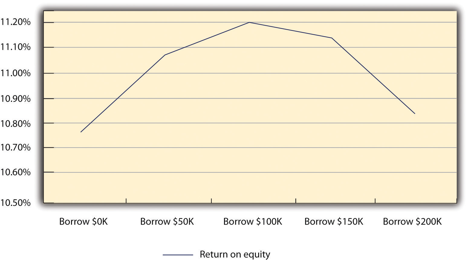
The owners then calculated the ROA and the ROE for the five scenarios (see Table 10.8 “ROA and ROE for the Five Scenarios”). When they examined these results, they noticed that the greatest ROA occurred when the new machinery was financed exclusively by equity capital. The ROA declined as they began to fund new machinery with debt: the greater the debt, the lower the ROA. However, they saw a different situation when they looked at the ROE for each scenario. The ROE was greater in each scenario where the machinery was financed either exclusively or to some extent by debt. In fact, the lowest ROE (the firm borrowed the entire $200,000) was 50 percent higher than if the firm did not acquire the new equipment. A further examination of the ROE results provides a very interesting insight. The ROE increases as the firm borrows up to $100,000 of debt. When the firm borrows more money ($150,000 or $200,000), the ROE declines (see Figure 10.3 “ROE for the Five Scenarios”). This is a highly simplified example of optimal capital structure. There is a level of debt beyond which the benefits measured by ROE begins to decline. Small businesses must be able to identify their “ideal” debt-to-equity ratio.
Table 10.8 ROA and ROE for the Five Scenarios
| Borrow $0 | Borrow $50,000 | Borrow $100,000 | Borrow $150,000 | Borrow $200,000 | |
|---|---|---|---|---|---|
| ROA | 10.77% | 10.50% | 10.04% | 9.41% | 8.59% |
| ROE | 10.77% | 11.07% | 11.20% | 11.14% | 10.84% |
Figure 10.3 ROE for the Five Scenarios
The owners decided to carry their analysis one step further; they wondered if the sales projections were too enthusiastic. They were concerned about the firm’s ability to repay any loan should there be a drop in sales. Therefore, they decided to examine a worst-case scenario. Such analyses are absolutely critical if one is to fully evaluate the risk of undertaking debt. They ran the numbers to see what the results would be if there was a 25 percent decrease in sales in 2011 rather than a 25 percent increase in sales compared to 2010. The results of this set of analyses are in Table 10.9 “Income Statement for the Five Scenarios Assuming a 25 Percent Decrease in Sales”. Even with a heavy debt burden for the five scenarios, the firm is able to generate a profit, although it is a substantially lower profit compared to if sales increased by 25 percent. They examined the impact of this proposed declining sales on ROA and ROE. These results are found in Table 10.10 “ROA and ROE for the Five Scenarios under the Condition of Declining Sales”.
Table 10.9 Income Statement for the Five Scenarios Assuming a 25 Percent Decrease in Sales
| Borrow $0 | Borrow $50,000 | Borrow $100,000 | Borrow $150,000 | Borrow $200,000 | |
|---|---|---|---|---|---|
| Revenue | $356,250 | $356,250 | $356,250 | $356,250 | $356,250 |
| Cost of goods sold | $195,938 | $195,938 | $195,938 | $195,938 | $195,938 |
| Gross profit | $160,313 | $160,313 | $160,313 | $160,313 | $160,313 |
| General sales and administrative | $71,250 | $71,250 | $71,250 | $71,250 | $71,250 |
| EBIT | $89,063 | $89,063 | $89,063 | $89,063 | $89,063 |
| Interest | $— | $3,750 | $10,000 | $18,750 | $30,000 |
| Taxes | $26,719 | $25,594 | $23,719 | $21,094 | $17,719 |
| Net profit | $62,344 | $59,719 | $55,344 | $49,219 | $41,344 |
Table 10.10 ROA and ROE for the Five Scenarios under the Condition of Declining Sales
| Borrow $0 | Borrow $50,000 | Borrow $100,000 | Borrow $150,000 | Borrow $200,000 | |
|---|---|---|---|---|---|
| ROA | 6.46% | 6.19% | 5.74% | 5.10% | 4.28% |
| ROE | 6.46% | 6.53% | 6.40% | 6.04% | 5.40% |
Video Clip 10.10
Debt Financing versus Equity Financing: Which Is Best for Us?
Overview of the benefits and dangers associated with debt financing and equity financing.
Video Clip 10.11
Capital Structure
Compares capital structure to a commercial aircraft.
Video Clip 10.12
Lecture in Capital Structure
Explains why capital structure matters.
Video Clip 10.13
The Capital Structure of a Company
Discusses the issue of long-term and short-term debt in capital structure.
KEY TAKEAWAYS
- A relatively simply model—breakeven analysis—can indicate what sales level is required to start making a profit.
- Financial leverage—the ratio of debt to equity—can improve the economic performance of a business as measured by ROE.
- Excessive financial leverage—too much debt—can begin to reduce the economic performance of a business.
- There is an ideal level of debt for a firm, which is its optimal capital structure.
EXERCISES
- A new start-up business will have fixed costs of $750,000 per year. It plans on selling one product that will have a variable cost of $20 per unit. What is the product’s selling price to break even?
- Using data from the business in Exercise 1, in its second year of operation, it adds a second selling facility, which increases the fixed cost by $250,000. The variable cost has now decreased by $2.50 per unit. What is the new selling price to break even?
- Using the example in Section 10.3.2 “Capital Structure Issues in Practice”, how would the ROA and the ROE change if economic conditions made borrowing money more expensive? Specifically, what would be the impact if the interest rate on $50,000 was 10 percent; $100,000, 15 percent; $150,000, 17.5 percent; and $200,000, 20 percent?
- Again using the example in Section 10.3.2 “Capital Structure Issues in Practice”, how much would sales have to decrease to threaten the business’s ability to repay its interest on a $100,000 loan?
10.4 The Three Threads
LEARNING OBJECTIVES
- Understand that effective and efficient financial management can enhance value provided to customers.
- Appreciate that effective financial management can improve the firm’s cash-flow position.
- Understand that the use of technologies can significantly reduce cost of operations and improve profitability.
Customer Value
In Chapter 2 “Your Business Idea: The Quest for Value”, Chapter 6 “Marketing Basics”, and Chapter 7 “Marketing Strategy”, there has been extensive discussion of the notion of market segmentation. By segmenting the market, one improves the probability that a business will be able to better serve particular customers’ needs and thus provide better customer value. From a financial perspective, there may be an equivalent notion of segmentation. Earlier discussions on market segmentation were centered on how a business could provide value to particular sets of customers. A subsequent stage of this analysis would be to examine how and if these customers can provide value to a business. No one is served if the business provides significant value to its customers but the business goes broke in the process. The financial equivalent of customer segmentation examines the profitability of different groups of customers. Some customer groups may be extremely profitable to a firm, while others produce nothing but losses. Identifying these different groups requires a commitment to accounting and a financial analysis of each customer base. The first step is to determine the margin provided by each customer group. In many cases, this is a bit of a challenge. It may require more extensive record keeping. The business may have to use activity-based costing systems. (Activity-based costing systems were developed in the late 1970s and the early 1980s.) This approach to accounting “is a process where costs are assigned due to the cause and effect relationship between costs and the activity that drives the cost.”Tiffany Bradford, “Activity-Based Costing,” Accounting @ Suite 101, accessed December 2, 2011, tiffany-bradford.suite101.com/activitybased-costing-abc-a52148.
Done properly, activity-based accounting can help a business identify the true costs for serving particular customer groups and therefore identify their real profit margins. A business may discover that some customer groups are actually a source of losses for the firm.
It should be pointed out that activity-based accounting is complex, difficult to implement, and, in some instances, does not conform to the requirements of generally accepted accounting principles. This might mean that a business would have to have two coexisting accounting systems, which may be too much of a burden for the small business.
Cash-Flow Implications
It should not be too surprising to find that good financial management can benefit tremendously when a firm’s cash flow is improved. Two areas where good financial management can help would be e-procurement and factoring. E-procurement involves managing the timing of invoices to customers and from suppliers to improve the cash flow of the firm.Peter Robbins, “E-Procurement—Making Cash Flow King,” Credit Control 26, no. 2 (2005): 23–26. The electronic handling of orders and their associated invoices assures that customers will receive their orders in a more timely fashion. E-procurement means that fewer personnel are required to take and handle orders. This can be a tremendous source of cash saving in and of itself. E-procurement should be on any supply chain management program of a business. We discuss supply chain management in Chapter 12 “People and Organization”.
Another area where good financial management can improve cash flow is factoring. The most common form of factoring is associated with a business’s accounts receivable. Trade credits involve purchasing and taking delivery of supplies now while planning to pay for it later. (See Section 10.1 “The Importance of Financial Management in Small Business” for a discussion of trade credits.) Three key numbers often identify trade credits: a discount rate for early payment, the time to pay to take advantage of the discount rate, and the date by which the entire bill must be paid. We underscore the kinds of the factoring with the following example.
A firm makes a large sale of supplies—$200,000. The trade credit program is 2/10/60. This means that the firm will give a 2 percent discount if the customer pays the entire $200,000 within 10 days and expects the payment of the entire $200,000 within the next 60 days. The firm knows that its customer never exercises the discount opportunity and always pays on the last possible date. Further, let us assume that this firm is having a problem with its cash flow. It would like to expedite payment as quickly as possible but does not expect that the customer will obtain a 2 percent discount by paying within 10 days. This firm could exercise the factoring option. This business goes to another firm that would provide as much as 80 percent of the cash receivable invoice immediately for small fee. In other words, the firm would receive $160,000 immediately rather than waiting 60 days. When its customer pays the bill, the firm would receive, in total, slightly less than the $200,000 but would have expedited the payment and thus aided its cash flow. Factoring can be an important element in improving the overall cash flow of any firm.
Digital Technology and E-Environment Implications
We identify four sources of capital in Section 10.1 “The Importance of Financial Management in Small Business”, one of which is internally generated funds. Businesses can increase the supply of capital money by becoming more operationally efficient. Improved operational efficiency can save any organization considerable amounts of money. Many start-ups, particularly those with some technological savvy, use technology to produce significant cost savings. This recognition of the vital role of technology as a cost-saving tool came to the forefront at a recent GeeknRolla conference in London. This conference brings together new business start-ups and potential investors. There is a heavy emphasis on how new businesses (and established businesses) can successfully integrate a variety of technologies and improve their operational efficiencies. As one participant in the conference, Michael Jackson, an investor, said, “Companies that are cottoning on quickly to these tools are doing very well, and they are taking business away from those who are too slow to adapt.”Sharif Sakr, “GeeknRolla: Tech Start-Ups Reveal Cost-Cutting Tips,” BBC Business, accessed December 2, 2011, www.bbc.co.uk/news/business-12962023.
The 2011 conference paid special attention to the concept of cloud computing. This term refers to having software programs and databases located on an outsourced site. As an example, rather than buying Microsoft’s Office Suite for every computer in a business, one could access a word-processing program, a spreadsheet program, or a database as needed. The firm would be charged for each use or a monthly fee rather than having to purchase an entire package. Chapter 9 “Accounting and Cash Flow”, Section 9.4 “The Three Threads” mentions that one can even access an entire accounting system as a part of a cloud computing option. As Sharif Sakr said, “In addition to being ‘pay-as-you-go,’ cloud computing has the advantage of reducing the number of computers, servers and network connections that a small business needs.”Sharif Sakr, “GeeknRolla: Tech Start-Ups Reveal Cost-Cutting Tips,” BBC Business, accessed December 2, 2011, www.bbc.co.uk/news/business-12962023.
In addition to reducing a small business’s initial commitment to an information technology (IT) infrastructure—computers, software, network systems, and IT staff—cloud computing provides some of the following additional benefits:
- Scalability. Many cloud applications allow for the growth of a business. As an example, some cloud accounting packages charge on the basis of the number of users; therefore, a company could purchase as much capability as it needed.
- Updates. Businesses do not have to worry about purchasing the latest version of the software, uninstalling the old version, and installing the latest version. This is done automatically by the vendor.
- Access. Cloud programs can be accessed wherever one has a connection to the Internet. A business is not tied to its own computer or the network where the software resides. This results in tremendous flexibility; as an example, one can access the program and the data while on the road with a client.
- Integration. Having programs and databases on the cloud facilitates multiple members of an organization successfully working together. No one has to worry whether he or she is working with the latest version of the spreadsheet or the client list.
- Security. Cloud providers recognize that securing their client’s data is a core issue for business survival. They will bring into play the required technology to ensure that every one’s data are secure and safe. They have much greater capability of assuring this than almost any small business.
- Customization. Businesses can acquire the software that they need.
- Extensions into the world of social media. More and more businesses are using various forms of social media—Facebook, Twitter, LinkedIn, and so forth—yet many small businesses lack the technological savvy to fully exploit these new avenues of marketing. Cloud providers can assist these businesses in this vital area.Eilene Zimmerman, “A Small Business Made to Seem Bigger,” New York Times, March 2, 2011, accessed December 2, 2011, www.nytimes.com/2011/03/03/business/smallbusiness/03sbiz.html?_r=1.
So how can smaller businesses aspire to efficiencies that much larger organizations have achieved through the use of IT while achieving it at a fraction of the cost? Entire accounting systems can be placed on the cloud. FreshBooks, which is free for solo location businesses, provides an accounting system that can be extended to allow business operators to submit invoices via the iPhone. Shoeboxed, another cloud-based company, allows small businesses to take digitalized receipts and turn them into invoices.
Owners and employees can more productively manage their time by using a variety of scheduling programs. TimeTrade is an effective personal scheduling assistant. It can show prospective clients available times and assist in arranging a scheduled appointment. Major companies, such as Microsoft and Google, provide cloud-based applications that can be employed by both large corporations and the smallest of businesses. Microsoft has an e-mail system—Exchange—that can be used by smaller businesses for fees as low as $50 per month. Google Voice can translate voice mail and e-mail messages and forward them anywhere in the world. Programs such as Mail-Chimp can send information packages to any or all of a business’s clients and then automatically post the same information on the company’s Facebook and Twitter sites.
KEY TAKEAWAYS
- Just as a business must identify what is of value to its customers, it should also determine how valuable its customers are to the business.
- It may not “pay” to attract and keep all customers.
- Techniques such as factoring accounts receivable may improve the cash flow of a firm.
- The use of cloud computing can significantly reduce costs and improve the financial position of a firm.
- Local, national, and international economic conditions can affect any firm. Businesses should plan on how to deal with major economic upheavals.
EXERCISES
- Search the Internet to find out about the availability and price of activity-based accounting software.
- Imagine your boss has asked you to prepare a small report on using factoring as an option in her auto parts business. Search the Internet to find out about the economics of factoring.
- Prepare a report on accounting and finance software packages available through cloud computing. Discuss their pros, cons, and pricing structures.